Cinema Camera Beautifiers

This study is focused on exploring nonlinear gamut transforms done by cinema cameras. Such transforms make images non-linear and damage most of the techniques used in virtual production such as keying, lighting calibration and LED wall to camera matching. Since these transforms are not publicly documented, the goal is to to characterize and model them. The article describes the methodology of measuring, canceling and re-applying such transforms.

Known approach to linearization.

Cinema camera raw profiles are packed with transfer functions. To make an image linear, we have to apply the inverse transfer function to the image. These transfer functions are publicly documented for most cameras.

Here are some references:

• SLog3
• ARRI LogC4
• Blackmagic Film Gen 5

However, it turns out that the transfer function is not the only non-linear operation done by cinema cameras. There is also a nonlinear gamut transform happening in the camera before the transfer function is applied. So the pipeline looks like this:

Sensor data (linear) -> Gamut transform (non-linear) -> Transfer function (non-linear) -> Encoded image

What is gamut nonlinearity?

Since light is additive, every mixture of two arbitrary colors must lie on a straight line between these colors. However, due to gamut nonlinearity, these mixtures are bent away from the straight line. In simple words, Half-Yellow(0.5 0.5 0) will not lie between Red(1 0 0) and Green(0 1 0). There is a reason why this nonlinear gamut transform exists, but that is a topic for another article.

Naming

Since I failed to find an established term for this transformation, I will call it a Beautifier as we call it internally at Antilatency. The inverse operation will be accordingly called a Debeautifier. The naming addresses the fact that this transform is equivalent to artistic color grading; there is no single “correct” way to do it. Sometimes this phenomenon is referred to as gamut compression. However, I would prefer not to blur the meaning of that term, since it currently describes a transformation with a specific mathematical form — unlike the more arbitrary transformations applied inside cameras. Later in this article, the shape of this transform will be shown, and it will become clear that it is not a simple gamut compression.

Why should we care about it?

Virtual production is a set of mathematical operations. Any mathematical operation becomes invalid once artistic color grading is applied. As I mentioned, Beautifier has its role, but it should be applied after all mathematical operations (e.g., keying, lighting calibration, display-to-camera mapping) are completed, at the end of the pipeline. Otherwise, these operations will produce incorrect results.

If the camera footage is at the end of the pipeline or is followed by artistic color grading only, then Beautifier can be applied in-camera. In Virtual production, however, camera footage is the input of the pipeline, so it is critical not to apply Beautifier at this stage, or to ensure it can be undone.

Several teams around the world have already found this problem while working in virtual production.

OpenVPCal @ Netflix

OpenVPCal is an open-source tool for camera and LED wall calibration in virtual production. The goal of the toolset is to be able to accurately predict a color captured by a camera from a color sent to an LED wall. In this presentation, the author explains a method to achieve better calibration results by using desaturated color patches for calibration. One of the reasons for that they mention is

Camera’s internal calibration might “bend” highly saturated colours “by design”.

CyberGaffer @ Antilatency

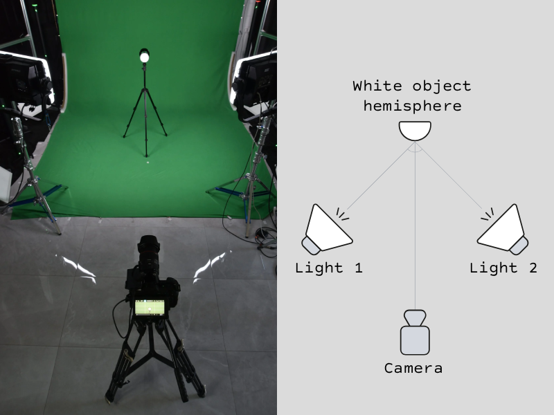
The first time I encountered this problem was during the CyberGaffer project, where accurate lighting calibration was required. During calibration, the software captures a reference white sphere illuminated by different light fixtures (per channel). The goal of the algorithm is to be able to predict the color of the sphere under any combination of lighting parameters. This is required to solve the inverse problem - to calculate lighting parameters for any given target illumination and configure physical lights accordingly. Independently, we found the same symptoms as the Netflix team did, and came to the same solution - to mix a portion of the white LED light into the R,G,B LEDs’ output to desaturate colors during the calibration, and later reconstruct the original saturated colors.

The problems with that approach are:

• We never know how much desaturation is enough to avoid nonlinearity problems.
• Desaturation reduces the determinant of the matrix, bringing the matrix axes closer to a collinear state. The smaller the determinant, the more noise and measurement inaccuracies will affect the calibration result, since to recover the original primaries from desaturated color patches, we need to multiply them by the inverted matrix. So we should be careful not to desaturate colors too much.
• This approach does not solve the problem.

It is a very good hack though, and later in this article I will explain why it works for some colors.

How can you spot gamut nonlinearity at home?

The Two Lights Experiment relies on the fact that light is additive. Therefore, for a truly linear camera, the photo of a scene illuminated by both lights must be equal to the per-pixel sum of images of the scene illuminated by each light separately. We can use this knowledge to check whether a camera is linear or not. The experiments can be done with minimal equipment.

You will need:

• A cinema camera
• 2 RGB lights
• A white object of any shape

First let’s capture 4 images (I1, I2, I3, I4), setting lights to one of two colors (states) as shown in the table below.

Image	Light 1	Light 2
I1	Black	Black
I2	White	White
I3	Black	White
I4	White	Black

Then we remove transfer function from these images, compute the two sums: I1+I2 and I3+I4, and compare them. If the camera were linear, those sums would be equal. Non-zero difference indicates nonlinearity.

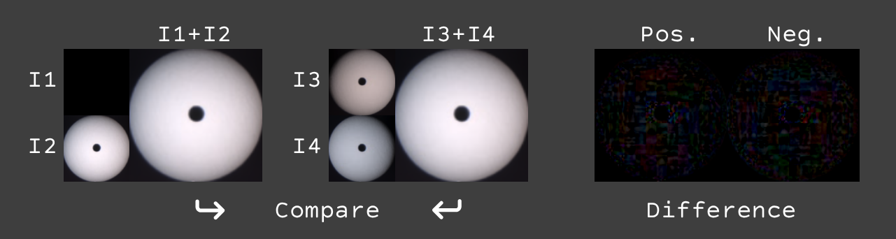As expected, the difference is very small (noise scale). That means that mixtures of black and white are linear.

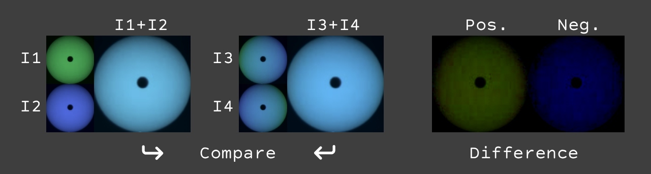
Now, let’s select another color pair for the next experiment: Red and Green. So our 4 images in this experiment are:

Image	Light 1	Light 2
I1	Red	Red
I2	Green	Green
I3	Red	Green
I4	Green	Red

Results for Red-Green:

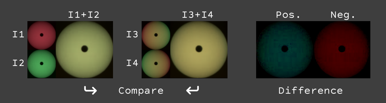
As we can see, there is a significant difference between these sums. That means that mixtures of Red and Green are nonlinear.

We can perform the same experiment for other color pairs as well.

Green-Blue: Blue-Red:

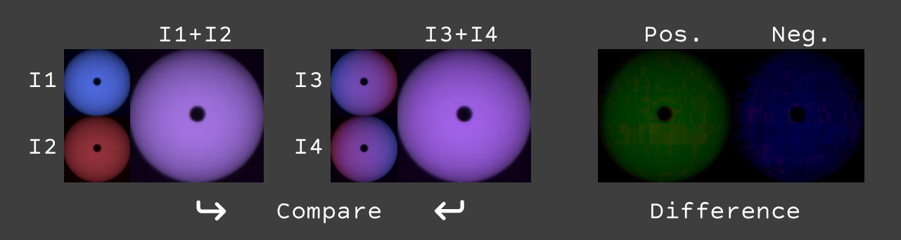
The same nonlinearity is observed there as well.

That experiment shows that the camera images are linear along brightness, but nonlinear across gamut plane.

Measuring and isolating gamut nonlinearity

The experiment above can only show that nonlinearity exists, but does not provide enough data to measure and characterize it. In order to do that, we’ve designed a measurement device that is able to precisely display linear colors. This device is based on RGB LEDs with excellent voltage stability and state-of-the-art PWM control.

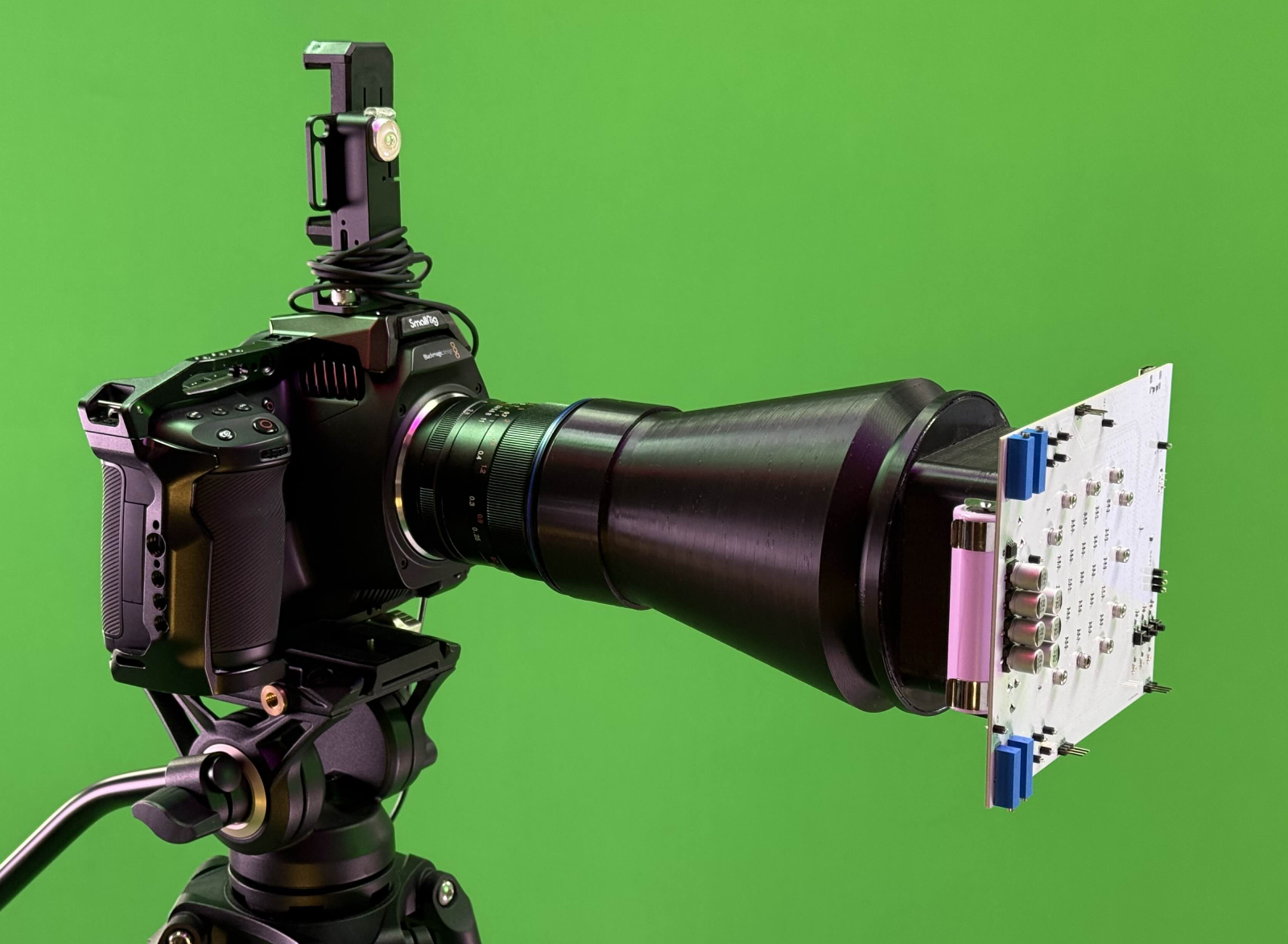This device is able to display temperature-balanced color sequences with high accuracy, allowing us to probe the camera’s response to various color stimuli.

Here is a calibration sequence fragment. The central area shows the color to be averaged later to reduce noise; four dots in the corners act as reference points for alignment and as a strobe to split the sequence into samples.

A 12-minute-long calibration video contains 16x16x16=4096 color samples covering the entire RGB cube uniformly.

Here is the measured data:

First, let’s remove transfer function.

As you can see in this plot, there are two transformations still present:

1. Matrix3x3 transform that is responsible for brightness, color balance and linear gamut shaping.
2. Some other nonlinear transform

Let’s remove Matrix3x3 transform as well. This lets us see only nonlinear transform. We will restore Matrix3x3 later in order to keep brightness and color balance and gamut unchanged.

This plot is Beautifier alone.

What is the general form of the Beautifier function?

From the Two Lights Experiment we already know that all of the colors between black and white are linear. This means that we are looking for a function that does not change linearity between these colors. Additionally, we can perform several more experiments for mixtures of black with different colors, and confirm that those mixtures are also linear.

This leads us to the conclusion that the function we are looking for is a Homogeneous function.

This means that if we scale input color by some factor and apply the function, it is equivalent to applying the function first and then scaling output by the same factor.

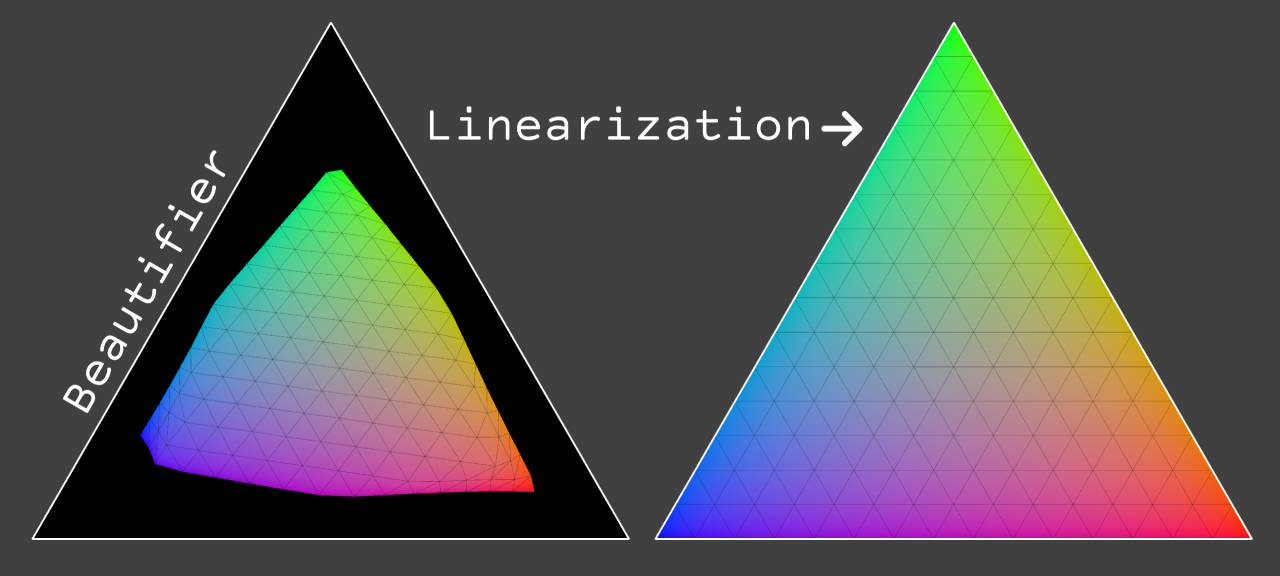
Visualizing a homogeneous transformation

To visualize a homogeneous transformation, we can slice through the RGB cube with a plane that passes through the red, green and blue points of the cube. Any distortions of the resulting triangle will represent the distortions of the entire cube, because all of the other colors will also lie on the scaled versions of this triangle.

To get such a slice, we can select samples where indices R+G+B=15 (our cube is 16x16x16 samples). Since all of the slices are similarly distorted, we can select any slice, but slice №15 has the highest resolution.

The white triangle on this plot represents an undistorted slice.

If you look closely at the shape of the distortion, you can notice that near the center (it represents less saturated colors) there is no distortion at all. This explains why the desaturation trick works and why it doesn’t. Using desaturated colors we can find a 3x3 matrix that will work well for the central region of colors, but as soon as we move to more saturated colors, the distortion becomes significant and matrix approximation fails.

In what way can these distortions be represented?

As we can see from the plot above, this distortion is unlike any smooth function such as polynomial or spline. It has an almost undistorted area in the center, with significantly distorted areas near the edges. Thus the best way to represent it is using a LUT-based approach. Technically, we can use a 3D LUT for this, but the problem of 3D LUTs is that the resolution of a 3D LUT decreases with brightness. If a 3D LUT has a size of 33x33x33 it has 32 steps between red(1,0,0) and green(0,1,0), but only 8 steps between dark-red(0.25,0,0) and dark-green(0,0.25,0). Another problem is memory consumption, for instance, to have 512 steps between red and green, we will need 512x512x512 = 134 million samples, that will take more than 1.6 GB of memory in binary form, and much more in text form.

Instead, we can invent a new type of LUT that is based on homogeneous coordinates. Such a LUT will have constant resolution across brightness levels, and will require much less memory.

Introducing 2D LUT

To have 512 steps between red and green, it uses 1.6Mb (not GB) of memory and has constant resolution across brightness levels. It can be stored as a simple 2D image. Since the shape of the described space is a triangle, we can pack it into a rectangle by cutting off a corner and flipping it.

If we display the gamut transform for the camera I used for this article as a 2D LUT, it looks like this:

Beautifier

Debeautifier (linearizer)

An important property of a 2D LUT is that it is a superset of Matrix3x3 transform. Any Matrix3x3 can be represented as a 2D LUT. The smallest 2D LUT of 3 pixels is actually a Matrix3x3 multiplication.

Previously, I mentioned that we removed Matrix3x3 transform to visualize the Beautifier alone. Since a 2D LUT includes Matrix3x3, we can represent a 2D LUT and Matrix3x3 transform together as a single 2D LUT.

Here is the result of removing the Beautifier from the original footage.

And here is the result of removing the Beautifier without restoring native color balance and brightness (Matrix3x3).

There are still some minor defects, and this is probably due to lack of resolution of measurements. As further increasing the measurement resolution would take too long to capture, the next step is to implement a hybrid measurement sequence with a basic resolution across the entire cube and a high resolution on the r+g+b=1 plane.

How Virtual Production pipeline should look like?

..for LED wall

• Get video from camera (beautified, packed with transfer function)
• Remove transfer function
• Remove Beautifier (apply Debeautifier)
• Calculate and apply Matrix3x3 to match LED wall primaries. In this stage of the pipeline any value sent to LED wall will be captured by camera with the same value. Of course, the display should be linear.
• Re-apply Beautifier on post if needed.

..for chroma keying

• Get video from camera (beautified, packed with transfer function)
• Remove transfer function
• Remove Beautifier (apply Debeautifier)
• Apply keying algorithm in linear space
• Composite foreground with linear background
• Re-apply Beautifier on post if needed.

Important note: When we re-apply the Beautifier at the last stage, we can use a Beautifier from a different camera! As long as these cameras share sensitivity spectrums and primaries are aligned (using matrix3x3 transform).

I hope this research will be obsolete one day

Ideally, all cinema cameras should provide an option to disable the Beautifier in-camera, so virtual production teams can get linear footage directly from the camera without the need to reverse-engineer these transforms. Also, it would be great to have vendor-provided beautifiers to be able to re-apply them to keep the original look.

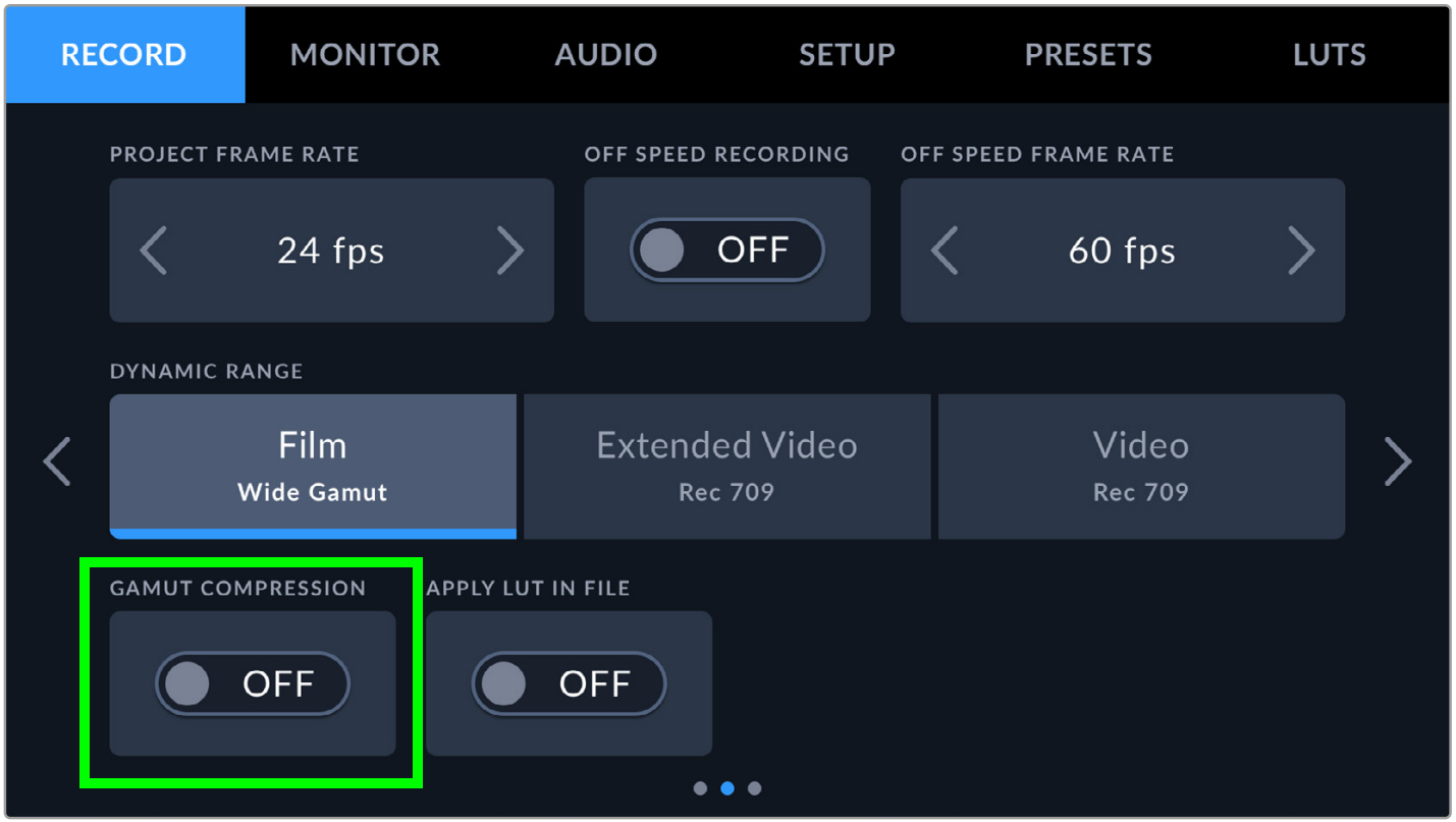
Today we can see some steps being taken in this direction. For instance, Blackmagic Design provides (since BRAW SDK Beta 3) an option to disable Gamut compresstion in BRAW SDK. BRAW format stores footage very close to sensor data and applies the Beautifier on the unpacking stage. Since version Beta 3, it is possible to disable this step and get footage without Beautifier applied. See BlackmagicRAW-SDK.pdf page 24. However, this does not help yet to get unbeautified video via HDMI/SDI outputs, required for virtual production. Moreover, to keep original color grading of the camera, we need a way to re-apply the Beautifier after all the virtual production operations are done, which is still not possible.

Dear color management system developers

It would be great if there was a standard way to describe the Beautifier/Debeautifier transforms, implemented in popular color management systems such as ACES, OpenColorIO, etc.